Simulating and fitting State-dependent speciation and extinction (SSE) models

library(diversitree)

Loading required package: ape

set.seed(117)

State-dependent speciation and extion (SSE) models are the subject of this set of exercises. The workhorse of these methods are the various flavors of birth-death models for generating trees.

Part 1: Simulating BiSSE models

So now, we are able to simulate trees using the birth-death process, and we learned earlier this week how to simulate trait evolution on a given tree. Now, we want to explore what happens if the tree generation process interacts with the traits. To do this, we will simulate Binary State Speciation and Extinction (BiSSE) models. We will start by simulating BiSSE models, then try fitting them (very similar to the basic birth-death model fitting).

BiSSE has 5 parameters: birth/diversification rates (lambda0, lambda1) corresponding to the two values of the trait (0 and 1); two death/extinction rates (mu0, mu1), and rates of the stochastic rate matrix, Q, (q01 and q10).

pars <- c(
    lambda0=0.1, 
    lambda1=0.2, 
    mu0=0.03, 
    mu1=0.03, 
    q01=0.01, 
    q10=0.01) 

tree <- tree.bisse(pars, max.taxa=50, x0=0)

State change information is available in tree$node.state, tree$tip.state, and tree$edge.state, but for plotting it is convenient to invoke the following:

plot(history.from.sim.discrete(tree, states=c(0,1)),
    tree, col=c('0'='black','1'='red'))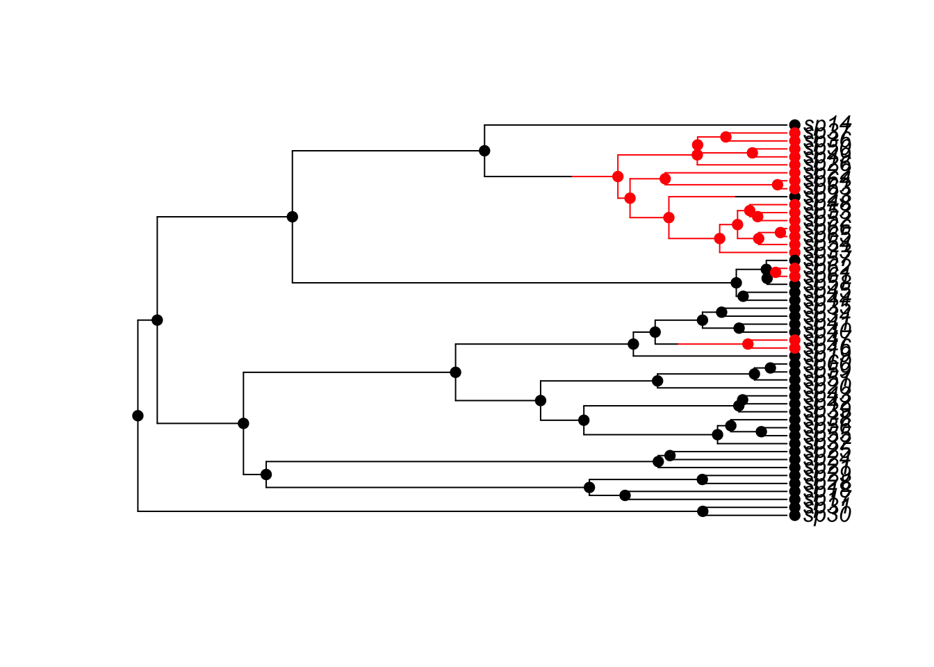 

The history.from.sim.discrete function accepts a tree produced by tree.bisse or tree.musse, and the states. The help pages indicate that the states should be 0 and 1 for BiSSE models. The history.from.sim.discrete object includes values for tip.state, node.state, history, discrete, and states:

names(history.from.sim.discrete(tree, states=c(0,1)))

[1] "tip.state"  "node.state" "history"    "discrete"   "states"    

I’m going to write a function to simulate and plot from parameter values I supply:

plotbissesim <- function(
    lambda0=1,
    lambda1=1,
    mu0=0,
    mu1=0,
    q01=1,
    q10=1,
    maxtaxa=50,
    x0=0){

    pars <- c(
        lambda0=lambda0, 
        lambda1=lambda1, 
        mu0=mu0, 
        mu1=mu1, 
        q01=q01, 
        q10=q10) 

    tree <- tree.bisse(pars, max.taxa=maxtaxa, x0=x0)
    plot(history.from.sim.discrete(tree, states=c(0,1)),
        tree, col=c('0'='black','1'='red')) 
    legend("topleft", 
           legend=c("state 0","state 1"), 
           col=c("black","red"), 
           lty=1, lwd=2, 
           bty="n", cex=0.8)
}

Because I supplied defualt values, this will just run:

plotbissesim()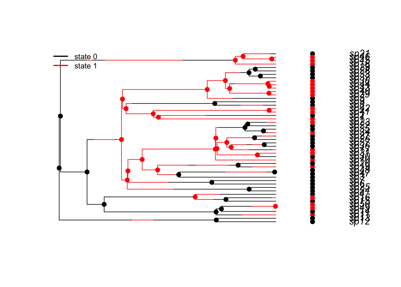

Or, I can tweak parameters (as many at a time as I want):

plotbissesim(lambda0=3)

plotbissesim(lambda0=0.1,lambda1=1,q01=.1,q10=1,x0=1)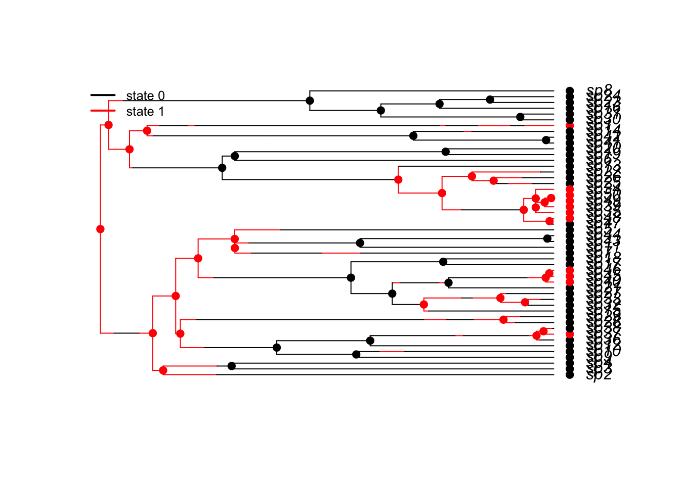

BiSSE Simulation Exercises:

1 .

Simulate a population that starts in a hostile environment but can move to a safer habitat with less predation. Assume the organisms are dumb (or just plants), so that individuals tend to spend the same amount of time in each habitat before moving to the other one. Do the simulations match your intuition about what should happen to the population in this scenario? Do you see different outcomes if migration is slow or fast relative to the birth and death rates? What happens if you simulate more taxa? (Try up to 10^4 or 10^5).

Also, try setting include.extinct=TRUE in your simulations to see how things change.

2.

Simulate a population that can move to a new habitat where there are more resources available, and organisms can produce more offspring. Assume that organisms have the same life expectancy in each area. You can also assume that individuals spend the same amount of time in each location. How does this scenario compare to the previous one, in terms of the trees you generate? Try different numbers of taxa.

3.

Now, suppose through no fault of their own that organisms are transported to a terrible environment at a much faster rate than they can escape. If you didn’t know the parameters you used, would it be obvious from the trees that one of the locations is worse than the the other?

4.

Supose the organisms are intelligent, and preferentially move to the location where there is less predation, and/or better resources. Do you think the phylogenies contain information about the crummy habitat?

5.

Try to simulate multi-state models using tree.musse. This example comes from the help page for ?tree.musse. Modify this to include 4 states with equal rates of movement between all of the states.

## A 3-state example where movement is only allowed between neighbouring
## states (1 <-> 2 <-> 3), and where speciation and extinction rates
## increase moving from 1 -> 2 -> 3:

pars <- c(.1,  .15,  .2,  # lambda 1, 2, 3
          .03, .045, .06, # mu 1, 2, 3
          .05, 0,         # q12, q13
          .05, .05,       # q21, q23
          0,   .05)       # q31, q32

set.seed(2)
phy <- tree.musse(pars, 30, x0=1, include.extinct=TRUE)

h <- history.from.sim.discrete(phy, 1:3)
plot(h, phy, cex=.7)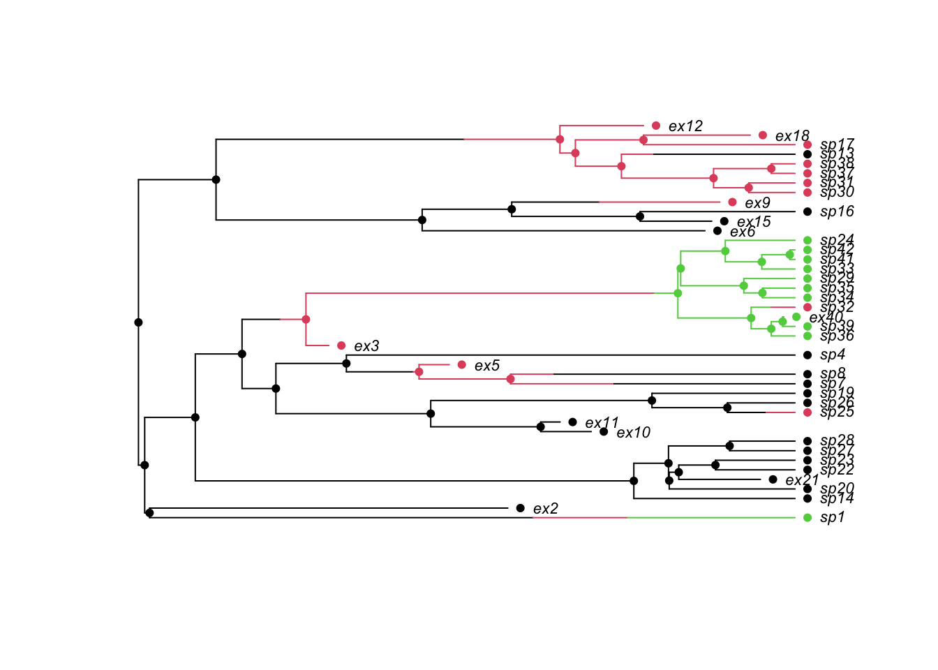

Modify this to include 4 states with equal rates of movement between all of the states.

Part 2: Fitting BiSSE models:

Now that we have some familiarity with the behavior of the BISSE model, we will try to use the model for parameter estimation, i.e. inference via model fitting.

Our goals are:

1. Learn how to specify a BiSSE model log-likelihood

2. Learn how to fit a BiSSE model

3. Learn how to constrain models to simplify models/estimate fewer parameters

4. Develop an intuition for how well we can estimate parameters in practice

Example: Benchmarking from simulations

Simulate a BiSSE tree:

pars <- c(
        lambda0=1,
        lambda1=5,
        mu0=0.8,
        mu1=0.8,
        q01=0.1,
        q10=0.12)

set.seed(117)
tree <- tree.bisse(pars, max.taxa=50, x0=0)

The make.bisse function is a scalar function of two variables of the form loglik = loglik(c(lambda,mu))

loglik <- make.bisse(tree, tree$tip.state)

What are the MLEs?

mles <- find.mle(loglik, pars)

# these are the parmeter values that this infers: 
print(mlepars <- mles$par)

     lambda0      lambda1          mu0          mu1          q01          q10 
5.170918e-01 3.708414e+00 3.894023e-09 8.022539e-01 3.424501e-01 5.801057e-02 

Let’s visualize the likelihood surface one parameter at a time (holding the other parameter at the MLE; not exactly profile likelihoods, but pretty close):

loglik_lambda0 <- function(lambda0) loglik(c(lambda0,mlepars[-1]))
loglik_lambda1 <- function(lambda1) loglik(c(mlepars[1],lambda1,mlepars[3:6]))

loglik_mu0 <- function(mu0) loglik(c(mlepars[1:2],mu0,mlepars[4:6]))
loglik_mu1 <- function(mu1) loglik(c(mlepars[1:3],mu1,mlepars[5:6]))

loglik_q01 <- function(q01) loglik(c(mlepars[1:4],q01,mlepars[6]))
loglik_q10 <- function(q10) loglik(c(mlepars[1:5],q10))

lambdavals <- exp( seq(-5,2,length=50))
muvals <- exp( seq(-9,2,length=50))
qvals <- exp( seq(-9,2, length=50) )

loglik_lambda0_vals <- sapply(lambdavals, loglik_lambda0)
loglik_lambda1_vals <- sapply(lambdavals, loglik_lambda1)

loglik_mu0_vals <- sapply(muvals, loglik_mu0)
loglik_mu1_vals <- sapply(muvals, loglik_mu1)

loglik_q01_vals <- sapply(qvals, loglik_q01)
loglik_q10_vals <- sapply(qvals, loglik_q10)

par(mfrow=c(3,2))

plot(lambdavals,loglik_lambda0_vals)
abline(v=pars['lambda0'],col='red')

plot(lambdavals,loglik_lambda1_vals)
abline(v=pars['lambda1'],col='red')

plot(muvals,loglik_mu0_vals)
abline(v=pars['mu0'],col='red')

plot(muvals,loglik_mu1_vals)
abline(v=pars['mu1'],col='red')

plot(qvals,loglik_q01_vals)
abline(v=pars['q01'],col='red')
plot(qvals,loglik_q10_vals)
abline(v=pars['q10'],col='red')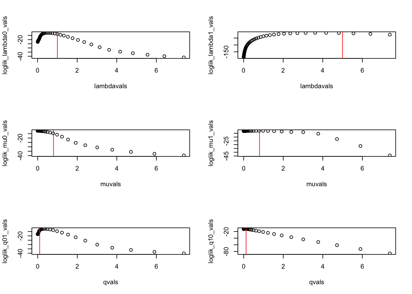

So, the parameters might be identifiable, but already this looks more challenging than the birth-death models we fit earlier today.

The MLE differs from the “true” values used to produce the simulation, but that is expected.

Of course, these approximations of profile likelihoods don’t show how correlated some of these parameters are with each other. We might as well use MCMC to do this:

This will take quite a lot longer than our birth-death model with just 2 parameters:

mcmc_fit <- mcmc(loglik, pars, nsteps = 1000, w=1) 

Looking at the different plots of the MCMC output, are you able to say which parameters that are more difficult to estimate than others?

Exercises

1.

What parameters seem to exhibit the highest correlations? The lowest? (You will need to plot all the pairwise combinations.) How do parameter estimates compare to the values used in the simulation? Is it easier to estimate one diversification rate or the other? Ditto for the mu’s and q’s. Why do you think that is?

2.

Increase the number of taxa in your tree. How does your ability to estimate parameters change? Does it become easier to estimate migration rates, or death rates? Using 200 taxa should be doable, but see how high you can go before computations get bogged down. Be sure to describe bias as well as precision of estimates.

3.

You may notice that the “data” (putting it in quotes b/c we simulated it) contain more information about one of the migration rates than the other. Which migration rate is it, and why do you think it might be easier to estimate it with greater precision than the other one? It might be helpful to plot the tree.

plot(history.from.sim.discrete(tree, states=c(0,1)),
                tree, col=c('0'='black','1'='red'))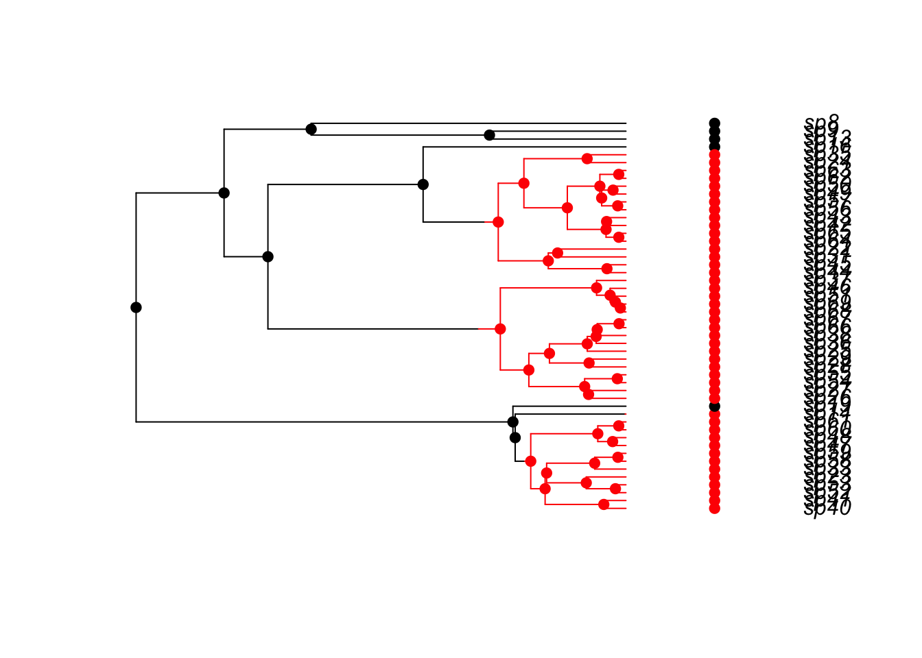

4.

Set migrations to be the same order of magnitude as the the diversification rates and repat the analysis. Does it always become easier to estimate q_ij?

5.

Set migration to be asymmetric. How easy is this to detect? You can start by assuming diversification and extinction rates are the same in each location.

6.

Under what circumstances do you think it is possible to reliably estimate extinction rates? Carry out an analysis to confirm or refute your hypothesis.

7.

Are there are any situations where it is difficult to estimate diversification rates? Comment on bias and variance.

8.

Naively, one might think that having larger differences between parameters (lambda0 vs lambda1, for example) would make estimation easier. Why is that not necessarily the case with BiSSE models? (Hint: what happens in simulations with large differences in diversification rates?)

9.

Try setting a constraint in the log-likelihood function that mu0=mu1. Does this help estimate the other parameters? Does it make it easier to estimate the overall exctinction rate (mu)?

Hint: it works like this: loglik_constrained <- constrain(loglik, mu0 ~ mu1)

`

Optional ensemble MCMC method

Let’s use an ensemble MCMC sampler from the package mcmcensemble. This implements an ensemble MCMC method that is well-suited to problems where paramters exhibit high correlation. If you’re interested, check out this paper:

Goodman J, Weare J. Ensemble samplers with affine invariance. Communications in applied mathematics and computational science. 2010 Jan 31;5(1):65-80.

library(mcmcensemble)

The make.bisse function will throw errors if we try to plug in negative parameters:

loglik(-pars)

For an MCMC routine that isn’t included in diversitree, we need to ensure that we can do an unrestricted search in parameter space.

loglik_transformed <- function(pars){
    pars <- exp(pars)
    loglik <- loglik(pars)
    return(loglik)
}

loglik_transformed(log(pars))
# This looks ok.

loglik_transformed(-log(pars))
# Calculates a value without error. Good to go.

nwalkers <- 100 #ensemble size
nsteps <- 50 #number of times to update entire nsemble

# initialize the ensemble:
mcmc_inits <- matrix(nrow=nwalkers, ncol=6)
for(i in 1:nwalkers) mcmc_inits[i,] <- jitter(log(mlepars))

# run the ensemble MCMC:
mcmc_fit <- MCMCEnsemble(loglik_transformed, 
    inits=mcmc_inits, 
    max.iter=nwalkers*nsteps, 
    n.walkers = nwalkers)

# Now, let's try to visualize the profile log-likelihoods (including
#   the curves we generated earlier):

par(mfrow=c(3,2))

plot(mcmc_fit$log.p ~ mcmc_fit$samples[,,1],xlab=bquote(lambda[0]))
#lines(log(lambdavals), loglik_lambda0_vals, col='red') 

plot(mcmc_fit$log.p ~ mcmc_fit$samples[,,2],xlab=bquote(lambda[1]))
#lines(log(lambdavals), loglik_lambda1_vals, col='red') 

plot(mcmc_fit$log.p ~ mcmc_fit$samples[,,3],xlab=bquote(mu[0]))
#lines(log(muvals), loglik_mu0_vals, col='red') 

plot(mcmc_fit$log.p ~ mcmc_fit$samples[,,4],xlab=bquote(mu[1]))
#lines(log(muvals), loglik_mu1_vals, col='red') 

plot(mcmc_fit$log.p ~ mcmc_fit$samples[,,5],xlab=bquote(q[0~1]))
#lines(log(qvals), loglik_q01_vals, col='red') 

plot(mcmc_fit$log.p ~ mcmc_fit$samples[,,6],xlab=bquote(q[1~0]))
#lines(log(qvals), loglik_q10_vals, col='red') 

In the vicinity of the MLE, the MCMC results should closely match the profile likelihood curves (but far away from the MLE there is no reason why they should be similar). (Why?)

Looking at the different plots, are you able to say which parameters that are more difficult to estimate than others?

What if we look at parameter correlations?