Fitting and simulating Markov models on trees using ancestral character estimation (ace)

rm(list=ls())

library(ape)
library(expm) # matrix exponential

Loading required package: Matrix

Attaching package: 'expm'

The following object is masked from 'package:Matrix':

    expm

The following object is masked from 'package:ape':

    balance

This code simulates output from the ace function. We will first try to grasp how the model behaves before we we try fitting it to data.

Ancestral character estimation methods can be based on a variety of approaches, but we will consider Markov chains superimposed on phylogenies. In the accompanying code to this we will learn how to fit these models using Maximum Likelihood, but for now we focus on simulating Markov chains on trees to understand how the models work.

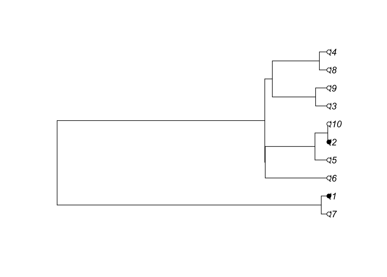
First, let’s simulate a tree and some tip states:

tree <- rcoal(10)
x <- sample(c(0,1), size=10, replace=T)

plot(tree)
tiplabels(pch=21,bg=x)

fit <- ace(x, tree, type='discrete', model='ARD')

Warning in sqrt(diag(solve(h))): NaNs produced

Exercise 1

Navigate through the ace help pages to determine whether Qij corresponds to the transition rate from state i-> j or from state j -> i. Based on your answer, does the Master equation for the Markov process use column or row vectors? Then, define a generator matrix, Q, in terms of the rates estimated just above (replacing the following line):

Q <- matrix(c(-1,1,1,-1),ncol=2) 
# can scale rates up or down:
Q <- Q/1

getP <- function(t,Q){
    P <- expm(Q*t)
    return(P)
} 

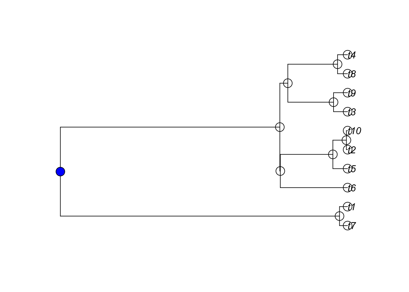
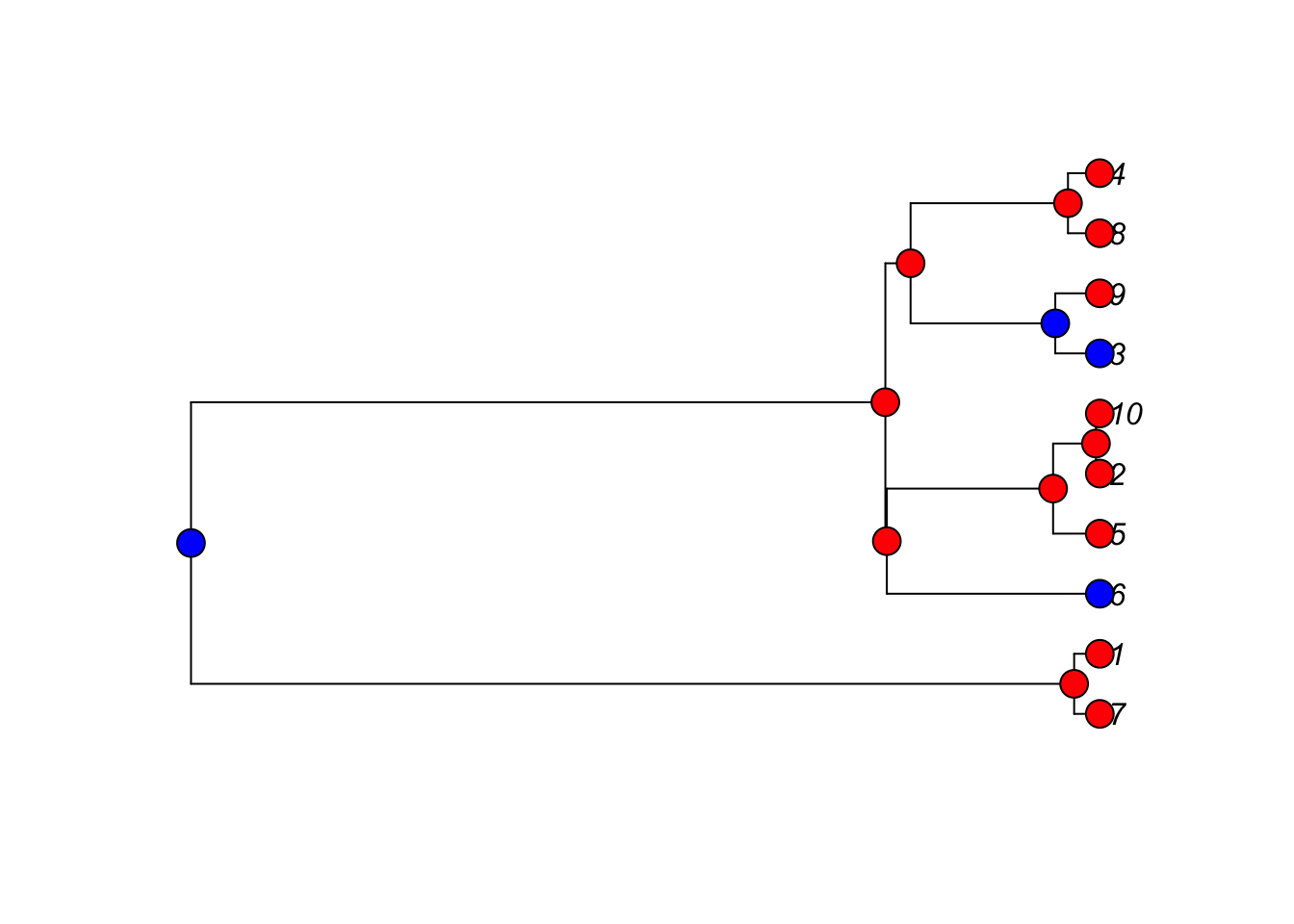
Now, we will start at the root of the tree and simulate states at the internal nodes and at the tips of the tree. (The ape package does not have a function to easily do this for us, but it is good exercise to practice it ourselves).

First, let’s create a vector to store all of the states we simulate:

states_vec <- rep(NA,(tree$Nnode + length(tree$tip.label)))
names(states_vec) <- c(tree$tip.label, paste0("node", 1:tree$Nnode))

Let’s just work with binary states for now:

states <- c(1, 2)
state_colors <- c('blue','red') #for plotting

Let’s assign a condition at the root; could be probabilities generally, but let’s say it starts in the first state with certainty for now:

pi_root <- c(1,0) 

Let’s start with the root state:

root <- length(tree$tip.label) + 1
states_vec[root] <- sample(states, 1, prob = pi_root)

Let’s plot this as we go:

plot(tree)
tip_states <- states_vec[tree$tip.label]
tiplabels(pch=21, bg=state_colors[tip_states], cex=2)
node_states <- states_vec[paste0("node", 1:tree$Nnode)] 
nodelabels(pch=21, bg=state_colors[node_states], cex=2)

We will do a preorder traversal, which starts at the root and descends down the tree to the tips:

preorder <- rev(postorder(tree))  # parent before children

The list of all of the edges of the tree is located in tree$edge:

edges <- tree$edge

Each row is an edge. The first column represents the parent, the second represents the descendant.

colnames(edges) <- c('parent','descendant')
edges <- as.data.frame(edges) # to use the handy $ command for columns

The entry in

tree$edge.length

is a vector of lengths for each of the edges; it corresponds to the same edges in tree$edge:

edge.lengths <- tree$edge.length

we start with the initial state at the root and use the Markov chain to sample subsequent states:

edges$parentstate <- states_vec[edges$parent]
edges$nextstate <- NA
edges$lengths <- edge.lengths

for(i in 1:nrow(edges)){
    parent_state <- if(edges[i,'parentstate']==1){c(1,0)}else{c(0,1)}
    prob = getP(edges$lengths[i],Q) %*% parent_state
    next_state <- sample(c(1,2), size=1, prob=c(prob))
    new_parent <- edges[i, 'descendant']
    edges[i,'nextstate'] <- next_state  
    edges[edges$parent==new_parent, 'parentstate'] <- next_state
}

Now fill in states_vec:

states_vec[edges$parent] <- edges$parentstate
states_vec[edges$descendant] <- edges$nextstate

Let’s plot this:

plot(tree)
tip_states <- states_vec[tree$tip.label]
tiplabels(pch=21, bg=state_colors[tip_states], cex=2)
node_states <- states_vec[paste0("node", 1:tree$Nnode)] 
nodelabels(pch=21, bg=state_colors[node_states], cex=2)

Exercises

1.

Simulate some tip states on a tree using a Markov model that you specify, and use ace to estimate it. Scale this up for a large number of tip state configurations to see how the distribution of Maximum Likelihood estimates for the Markov model rates compare with the true values you supplied. Are there particular combinations of branch lengths and rates that make it difficult to estimate model parameters?

2. (Hard, or maybe impossible)

Modify the code above to condition on a particular tip state configuration. This way, we can observe distributions of evolutionary scenarios consistent with a particular set of observations.

3.

In a fitted ace object, there is an element called lik.anc which records the probability of ancestral states at each node of the tree. Plot a dataset of your choice with pie charts displaying the ancestral state probabilities associated with models that you fit using ace. Navigate through the help pages (?ace) to specify a few different versions of models that impose constraints on the Markov generator, Q. How sensitive are ancestral state probabilities to your modeling choices?